


new sewer line was being installed at a manufacturing plant. The plan was to excavate the proposed route and lay the utility in the trench. It was known that many buried utilities existed in the vicinity, and they did not want to have any utility strikes during the installation process.
Challenges
Some very old as-built drawings showed buried utilities made of metal, plastic and concrete. However, the landscape had changed dramatically since the drawings were done, so their position could not be trusted.
As this was on private property, the public one–call service could not be used, so a private locating company was hired to locate the existing utilities prior to construction.
Solution
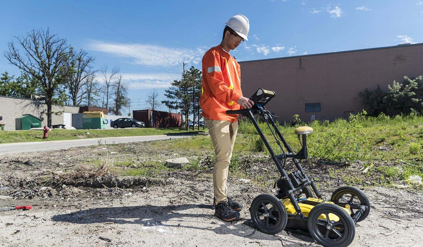
The project deliverable included marking the utilities on the ground, and delivering a report detailing the findings to the manufacturing plant. Given the variability with types of utilities, their depth and material composition, the locating company decided to use an LMX200™ Ground Penetrating Radar (GPR) system with GPS.
Locating utilities in areas with densely packed installations can be a challenge, as was the case at this site. To get an accurate image of the location, depth, and orientation of the utilities, a 20ft by 20ft grid was laid out over the area of interest and a survey was completed as illustrated in Figure 1.

The first way to view the data is by looking at the cross–sectional data (sometimes called the raw data). The inverted U responses, called hyperbolas, indicate a reflected object from the ground. There are a large number of utilities (hyperbolas) visible in the cross–sectional data (Figure 2). A graphical representation of the pipes is shown in Figure 3 to make it easier to visualize. When lines are collected in a grid pattern they can be used to build depth slices (Figure 4) which is especially useful in complex situations with many targets.
 and XLine (right) show many hyperbolas, indicating a large number of targets.")

Depth slices show a top–down view of the GPR data collected in the grid, and can be sliced into at different depths. Depth slices can be viewed in the field directly on the LMX200™ display unit, or opened in the EKKO_Project™ GPR processing software.
The depth slices show that there are utilities at different depths, and that some utilities are joined by a T–junction. The position, depth, and orientation of all the utilities in the surveyed area are visible in the depth slices.

Some highlights from the depth slices:
- Pipe 4 is well defined in the 1.75 – 2.00 ft depth
slice. - The T–junction between pipes 1 and 3 is visible in the 2.50 – 2.75 ft depth slice.
- Pipe 5, is visible in the 4.00 – 4.25 ft depth slice, just below pipe 3, confirming the second hyperbola in the cross–section.
The depth slices were exported from the EKKO_Project™ GPR software and plotted using 3D visualization software (Figure 5). This allowed all GPR data to be displayed in a single view for easier interpretations. Users can rotate and cut into the data volume, or make weaker GPR signals translucent or invisible to highlight signals from strong reflectors.
Another output generated from EKKO_Project™ was an Interpretation Map (Figure 6). This is created by placing colored dots (or Interpretations) on the hyperbolas in Line Scan mode. The resulting map helps show the linearity of pipes, and is another way to visualize the data. These interpretations can be exported into third–party GIS software.


Results
Using the GridScan mode, the LMX200™ was able to easily locate all the buried utilities at varying depths down to 6 feet, and bring clarity to an otherwise congested area. By using other sources of information and surface visual clues, it was possible to identify the types of utilities located. As it turned out, the proposed path would have crossed a utility. As a result of these findings, the sewer trench route was shifted over slightly to avoid any possible conflict.


