GPR FAQ

Ground Penetrating Radar (GPR) is the general term applied to techniques which employ radio waves, typically in the 1 to 1000 MHz frequency range, to map structures and features buried in the ground (or in man-made structures). Historically, GPR was primarily focused on mapping structures in the ground; more recently GPR has been used in non-destructive testing of non-metallic structures.

The concept of applying radio waves to probe the internal structure of the ground is not new. Without a doubt, the most successful early work in this area was the use of radio-echo sounders to map the thickness of ice sheets in the Arctic and Antarctic and sound the thickness of glaciers. Work with GPR in non-ice environments started in the early 1970s. Early work focused on permafrost soil applications.

GPR applications are limited only by the imagination and availability of suitable instrumentation. These days, GPR is being used in many different areas including locating buried utilities, mine site evaluation, forensic investigations, archaeological digs, searching for buried landmines and unexploded ordnance, and measuring snow and ice thickness and quality for ski slope management and avalanche prediction, to name a few.

How does it work?

1. Emits weak radio frequency signals
2. Detects the echoes sent back and uses them to build an image
3. Displays signal time delay and strength

GPR is just like a fish finder & echo sounder

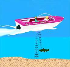
1. The finder sends out a ping
2. Signal is scattered back from the fish
3. Signal is scattered back from the bottom

1. As the boat moves it collects recordings
2. The recordings are displayed side by side
3. The result looks like a cross section

GPR Exploration Depths

Exploration depth is site specific

• soils absorb radio waves
• sands and gravel are favorable for GPR
• fine-grained soils such as silt and clay absorb signals
• salty water is totally opaque

What’s so tough about GPR?

1. The ground is more complicated
2. Man-made structures are complex
3. Some things simply do not reflect
4. Some grounds absorb all of the signals

Why doesn’t the pipe look like a pipe?

• the GPR record is a pseudo image of the ground
• localized features become hyperbolas (inverted V’s)
• the GPR sends signals into the ground in all directions
• echoes are observed from all directions
• closest approach (over target) occurs at the apex of V
• the shape of inverted V helps determine the exact depth

“How deep can You see?” is the most common question asked of ground penetrating radar (GPR) vendors. While the physics is well known, most people new to GPR do not realize that there are fundamental physical limitations.

Many people think GPR penetration is limited by instrumentation. This is true to some extent, but exploration depth is primarily governed by the material itself and no amount of instrumentation improvement will overcome the fundamental physical limits.

What controls penetration?

Radio waves do not penetrate far through soils, rocks and most man-made materials such as concrete. The loss of radio reception or cell phone connection while driving a car through a tunnel or into an underground parking garage attests to this.

The fact that GPR works at all depends upon very sensitive measuring systems being used and specialized circumstances. Radio waves decrease exponentially and soon become undetectable in energy absorbing materials, as depicted in Figure 1.

Figure 1: GPR signals decay exponentially in soil and rock.

The exponential attenuation coefficient, a, is primarily determined by the ability of the material to conduct electrical currents. In simple uniform materials this is usually the dominant factor; thus a measurement of electrical conductivity (or resistivity) determines attenuation.

In most materials energy is also lost to scattering from material variability and to water being present. Water has two effects; first, water contains ions which contribute to bulk conductivity. Second, the water molecule absorbs electromagnetic energy at high frequencies typically above 1000 MHz (exactly the same mechanism that accounts for why microwave ovens work).

Attenuation increases with frequency as depicted in Figure 2. In environments which are amenable to GPR sounding there is usually a plateau in the attenuation versus frequency curve which defines the “GPR window”.

Figure 2: Attenuation varies with excitation frequency and material. This family of graphs depicts general trends. At low frequencies ( 1000 MHz) water is a strong energy absorber.

Can I decrease frequency to improve penetration?

Lowering frequency improves depth of exploration because attenuation primarily increases with frequency. As frequency decreases, however, two other fundamental aspects of the GPR measurement come into play.

First, reducing frequency results in a loss of resolution. Second, if frequency is too low, electromagnetic fields no longer travel as waves but diffuse which is the realm of inductive EM or eddy current measurements.

Why can’t I just increase my transmitter power?

One can increase exploration depth by increasing the transmitter power. Unfortunately, power must increase exponentially in order to increase depth of exploration.

Figure 3: When attenuation limits exploration depth, power must increase exponentially with depth.

Figure 3 shows the relative power necessary to probe to a given depth for the attenuations depicted in Figure 1. One can readily see increases in exploration depth require large power sources.

In addition to practical constraints, governments regulate the level of radio emissions that can be generated. If the GPR transmitter signals become too large, they may interfere with other instruments, TVs, radios, and cell phones. (Unfortunately, these same ubiquitous devices are usually the limiting sources of noise for GPR receivers!)

Can I predict exploration depth?

Yes, provided the material to be probed is known electrically, many numerical calculation programs are available. The simplest way to get estimates of exploration depth is to use the radar range equation (RRE) analysis. Software to carry out these calculations is available and there are numerous papers on the subject. The basic concepts are depicted in Figure 4.

Figure 4: Radar range, shown here in flowchart form, determines energy distribution and provides a means of estimating exploration depth.

RRE analysis is very powerful for parametric studies and sensitivity analyses.

Radar Range is Too Complicated!

Many users say RRE is too complicated for routine use. If you don’t like to get into detailed calculations, we suggest using the following simpler rule-of-thumb for estimating exploration depth

D= 35/ meters

where is conductivity in mS/m. While not as reliable as the RRE, this helpful rule is quite useful in many geologic settings.

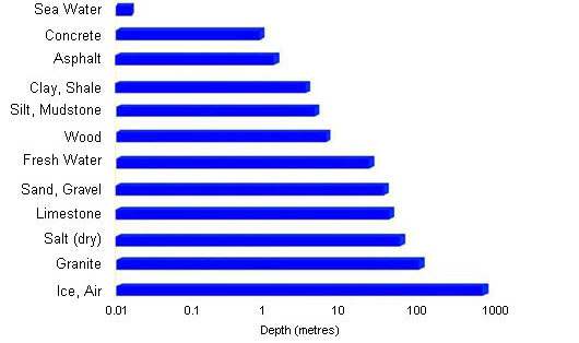
An even simpler approach is to use a table or chart of exploration depths attained in common materials. An example chart for common materials encountered with GPR is shown in Figure 5.

Figure 5: Chart of exploration depths in common materials. These data are based on “best case” observations. As Figure 9 demonstrates, material alone is not a true measure of exploration depth.

Figures 6, 7 and 8 show examples which range from deep to shallow exploration. Material type can be seen to control exploration depth. Unfortunately, exploration can not always be predicted by knowing only the material in the survey area.

Figure 6: Data from a massive granite – reflections are fractures. 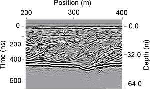Figure 7: Data showing bedding in wet sand deposits. Figure 8: Data shows response of barrels in wet, silty clay.

Figure 9 shows a section where the geology is basically uniform but the depth of exploration is highly variable. Pore water conductivity is varying while the geologic material is invariant! In this case, knowing conductivity provides a better measure of exploration depth than knowing the material.

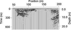Figure 9: GPR section from sand setting. Depth of exploration is determined by pore water conductivity-not the sand material. Contaminants leaching from a landfill cause variable conductivity (and exploration depth) with position.

Ground penetrating radar (GPR) measurements, such as shown in Figure 1, detect reflected or scattered energy. In technical jargon, reflections are created by changes in the electromagnetic impedance associated with property variations. Unfortunately, many GPR users are not familiar with the more esoteric aspects of radio fields and material properties.

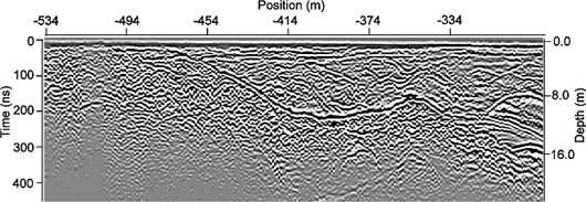Figure 1: Classic data set showing reflections from objects present in the survey area.

What are material properties?

“Material properties” characterize the physical attributes of a material. These properties range from density, elasticity, porosity, thermal conductivity, color, fabric, and texture to a host of other properties. The physical properties important for radio waves are dielectric permittivity, electrical conductivity and magnetic permeability.

GPR responds to changes in electrical and magnetic properties. People naturally tend to characterize a target by its visual or mechanical properties (i.e. directly sensed by sight, touch, etc.). A correlation often exists between electrical and other physical properties; hence GPR responses often conform to people’s preconceptions.

Why are electrical properties important?

Electrical properties control how electromagnetic waves travel through a material; dielectric permittivity primarily controls wave speed; and conductivity determines the signal attenuation.

Radar reflections occur when the radio waves encounter a change in the velocity or attenuation. The bigger the change in properties the more signal reflected.

Many GPR concepts are derived from optics. For example, Snell’s law describes the bending of both light rays and radio waves at a boundary between materials depicted in Figure 2. Bending (or refraction) depends on the change in wave speed between the materials.

Just as in optics, radio waves are partially transmitted and partially reflected at boundaries and the Fresnel reflection coefficient describes both light and radar waves.

Figure 2: Radar waves partially transmitted and reflected at boundaries. Rays also change direction crossing the boundary.

What are Fresnel coefficients?

Fresnel reflection coefficients quantify the amplitude of reflected and transmitted signals at boundaries. The ratio of the reflected-to-incident signal amplitudes is the reflection coefficient; the ratio of the transmitted-to-incident signal amplitudes is the transmission coefficient.

Reflection coefficients depend on the angle of incidence, the polarization of the incident field, and the velocity contrast. Figure 3 illustrates the variation of the reflection coefficient versus angle of incidence and polarization for a GPR wave incident at the water table where a velocity contrast of 1.6:1 might occur.

Figure 3: Amplitude of reflected signals depends on velocity contrast, direction of incidence, and polarity. The reflections for both polarizations at a water table are depicted.

Most situations are not this simple; reflector size and shape are also important. Purists argue that reflections are abstractions and that all responses are scattering responses. Fresnel reflection coefficients implicitly assume a planar and very extensive interface. This is seldom true in reality.

How are irregular shapes treated?

Some common sources of radar responses are depicted in Figure 4. Rough boundaries, localized features, long thin pipes and cables are all much more common than the planar boundary.

Figure 4: Common GPR targets can have a variety of geometries and spatial scales.

Geometry becomes important when boundary geometry dimensions approach the same size as the radar signal spatial dimension (i.e. wavelength). When this occurs, targets must be viewed as collections of scattering points that each capture and re-radiate some of the incident signal. These individual scatterers interact with one another to enhance or reduce re-radiated energy. Scatterers are characterized by their radar cross-section and a back-scatter gain.

What are GPR Cross-Section and Back-Scatter Gain?

The cross-section is a measure of the effective area that a scatterer projects into the path of the incident radar signal. The incident radar wavefront energy per unit area multiplied by the cross-sectional area determines the energy the scatterer extracts from the incident wave.

Figure 5: Illustration of scattering cross-section area and back-scatter gain. In (a) a large area is presented and most energy directed back. In (b) the target presents a small cross-section and the scattered signal is not directed back to the receiver.

The energy extracted signal can be absorbed or re-radiated in any direction. Back-scatter gain measures the amount of energy re-radiated back in the direction of the incident signal as depicted in Figure 5.

Back-scatter gain and cross-sectional area are either computed from numerical modeling or measured for standard geometrical shapes in laboratories. Some simple geometries yield relatively compact analytical back-scatter gain formulas.

The cross-sectional area is a function of the true geometrical cross-section of an object as well as the contrast in electrical properties. The back-scattered gain is primarily controlled by the geometrical attributes of the object.

What does all This Mean?

In a nutshell, radar responses are a function of both physical property contrast and geometry. The response of a sphere, as depicted in Figure 6, illustrates this concept.

Figure 6: Scattering from a spherical body as a function of sphere dimensional. For a small sphere, size dominates. For a large sphere, the response approaches a planar target.

For small objects the amount of energy scattered increases as the fourth power of the target dimension. When the target gets large, the response plateaus out and approaches that of a planar boundary (i.e. the Fresnel reflection coefficient). Between the extremes, the response will oscillate due to constructive and destructive interference within the target.

Frequency selection is controlled by two survey requirements – exploration depth and resolution length, as shown in Figure 1. Resolution length indicates the ability to uniquely identify closely spaced targets. More details on resolution length can be found in the January 2003 EKKO_Update.

Figure 1: Frequency selection is controlled by exploration depth and resolution length, D Z.

Exploration depth depends on many site specific factors with the most important being the signal attenuation rate in the host material. Attenuation rate depends on GPR frequency as indicated in Figure 2.

Figure 2: Attenuation dictates exploration depth. In an ideal material, attenuation plateaus above the transition frequency. In real environments, water or volume scattering cause attenuation to increase with frequency. The on-set of high frequency losses is very site specific.

In an ideal material, attenuation plateaus at high frequency. In real materials, heterogeneity and water relaxation absorption increase attenuation at high frequency. Scattering losses, as illustrated in Figure 3, always occur. A street lamp in fog is a good analogy. Water drops scatter the light resulting in greatly reduced visibility (i.e. light penetration is decreased).

Figure 3: GPR signals are scattered by small heterogeneities in material properties which reduce the transmitted signal.

Resolution length varies proportionately with GPR frequency since system bandwidth equals center frequency for impulse or baseband GPRs, as depicted in Figure 4.

Figure 4: Spatial resolution versus frequency length. Material velocity changes spatial resolution.

Figures 2 and 4 illustrate the dilemma: as GPR frequency increases, resolution increases but the exploration depth decreases. The compromise solution has a logical but not always unique solution.

Plotting exploration depth versus frequency, as shown in Figure 5, provides the basis of this discussion. For simplicity, exploration depth is selected to be three attenuation lengths in the material. Attenuation length is the inverse of attenuation rate and often referred to as skin depth.

Figure 5: Exploration depth (assumed to be three attenuation lengths) varies with frequency. The decrease in exploration depth at high frequency limits the upper practical GPR frequency.

As shown in Figure 6, the GPR bandwidth must lie between the shaded areas where GPR is not an appropriate method (dispersion is just too great). For maximum resolution fc is selected such that the upper edge of the GPR bandwidth touches the exploration depth curve. In some situations, a range of resolutions and center frequencies can be selected (Figure 7) while some situations leave little choice (Figure 8).

Figure 6: On a log scale, GPR bandwidth and, hence, resolution increase and decrease as center frequency is changed. The highest resolution (smallest resolution length) is achieved when the upper edge of the bandwidth box touches the exploration depth curve at the desired exploration depth. Figure 7: The GPR frequency can be placed anywhere in the unshaded region, as depicted in the figure. As the center frequency is decreased, the bandwidth, B, decreases resulting in lower resolution. Figure 8: In some cases, there is no choice about frequency, as shown here. As the heterogeneity scale length increases, the high frequency cut off moves lower.

The following is a simplified algorithm which can be coded in a spreadsheet and used to estimate fc based on this logic. (a) Characterize the site by estimating local relative permittivity, K, low frequency conductivity, , and heterogeneity scale, L (typical length of local variability in the host material). (b) Compute the exploration depth (see Figure 5).

(c) Specify the desired exploration depth, D (must be less than dplat). (d) Estimate high frequency limit factor for scattering

(e) Estimate maximum resolution ratio

using

(f) If R < 1, GPR is inappropriate. (g) If R > 1 then the GPR center frequency that gives the fairest depth versus resolution length compromise is:

If the host is very wet (high water content > 5%), then fc should be limited to less than 1500 MHz if the computed value is greater.

These results are upper limits on frequency. Not included in this simple analysis is the fact that GPR system power and sensitivity tend to increase with decreasing frequency. Using a somewhat lower frequency than computed is often a wise choice.

Accurately determining the depth of a reflection in a GPR data record requires knowledge of how fast the signals travel in the material under investigation. Several techniques are used such as CMP (common mid-point), WARR (wide angle reflection and refraction), known-depth-target, hyperbolic fitting to a local target and diffraction tail matching.

All of these techniques require GPR measurements along a traverse where the geometry is varying in controlled fashion. In other words, the distance to a target varies such that estimates of velocity can be extracted.

Figure 1: The GPR traverse should be perpendicular to the pipe or cable strike direction.

For pipe and cable location, or, in the Conquest example of rebar and conduit location, long linear features are localized targets if the GPR system traverses perpendicular to the feature alignment (Figure 1). To estimate velocity, the path length to the object must vary.

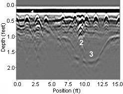
Figure 2: Plan view looking down on ground from above. Traverse 1 is perpendicular to strike and is optimal for velocity determination. Traverse 2 is at an oblique angle and traverse 3 is parallel to the pipe strike axis. Data from traverses 2 and 3 are not suitable for determining velocity.

Figure 2 illustrates this using a straight pipe or cable as an example. In order to extract velocity information, the radar system must be moved perpendicular to the axis of the pipe or cable. The long-axis direction is commonly called the “strike direction” or “strike” for short. If a GPR traverses perpendicular to the strike, the distance varies from the radar system to the pipe in a regular fashion. Traversing parallel to the pipe strike yields no change in the distance of the pipe and hence, a flat, non-changing event on the GPR record. Figures 3 and 4 show these two extremes using real data from a drainage pipe in a farm field.

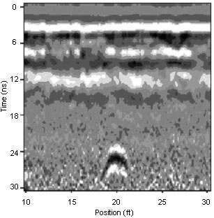Figure 3: GPR data over a clay drainage pipe perpendicular to pipe direction (line 1 in figure 8) 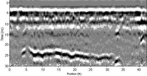Figure 4: GPR data over a clay drainage pipe parallel to pipe direction (line 3 in figure 8).

GPR cross-sections display signal amplitude versus position (normally on the horizontal axis denoted as x) and time (which is normally the vertical axis denoted as T). A local target has a travel time versus position as depicted in Figure 5. The mathematical form is a hyperbolic shape (inverted U on a GPR section) relating spatial position (x) to travel time (T). Figure 6 shows the response in a GPR cross-section as the target depth is varied while in Figure 7 the velocity is changed for a fixed depth.

Figure 5: Relationship between GPR position (x), object depth (d) and travel time (T). To is travel time when GPR is directly over the object. Figure 6: Schematic variations in GPR response when object depth is varied for constant velocity. Figure 7: Schematic variations in GPR response when velocity is varied for a fixed object depth.

A handy interpretation aid is to visually fit a model hyperbolic shape to the GPR data as illustrated in Figure 8. Placing the top of the model (triangle point) over the apex (top of inverted U) in the data section selects To. Adjusting the model shape to match the data yields an estimate of the velocity, v. Combining v and To yields an estimate of the depth to the top of the target.

Good field practice entails several traverses over an object. Only use the hyperbolic fitting on the traverse that gives the steepest slope to the arms of the inverted U. This approach assures getting the most correct velocity. A traverse not perpendicular to strike (line 2 in Figure 8) will always yield a velocity higher than the true velocity and the object depth will appear deeper than reality.

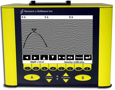Figure 8: Example of shape fitting to a target response on the DVL screen in the field. This feature is standard on Noggin, Conquest and pulseEKKO systems.

Radio frequency electromagnetic fields may pose a health hazard when the fields are intense. Normal fields have been studied extensively over the past 30 years with no conclusive epidemiology relating electromagnetic fields to health problems. Detailed discussions on the subject are contained in the references and the Web sites listed below.

The USA Federal Communication Commission (FCC) and Occupational Safety and Health Administration (OSHA) both specify acceptable levels for electromagnetic fields. Similar power levels are mandated by corresponding agencies in other countries. Maximum permissible exposures and time duration specified by the FCC and OSHA vary with excitation frequency. The lowest threshold plane wave equivalent power cited is 0.2 mW/cm2 for general population over the 30 to 300 MHz frequency band. All other applications and frequencies have higher tolerances as shown graphically in Figure 1.

Figure 1: FCC limits for maximum permissible exposure (MPE) plane-wave equivalent power density mW/cm2.

All Sensors & Software Inc. pulseEKKO, Noggin® and Conquest™ products are normally operated at least 1 m from the user and as such are classified as “mobile” devices according to the FCC. Typical power density levels at a distance of 1 m or greater from any Sensors & Software Inc. product are less than 10-3 mW/cm2 which are 200 to 10,000 times lower than mandated limits. As such, Sensors & Software Inc. products pose no health and safety risk when operated in the normal manner of intended use.

References

1. Questions and answers about biological effects and potential hazards of radio-frequency electromagnetic field.

USA Federal Communications Commission, Office of Engineering & Technology

OET Bulletin 56 (Contains many references and Web sites)

2. Evaluation Compliance with FCC Guidelines for Human Exposure to Radio Frequency Electromagnetic Fields.

USA Federal Communications Commission, Office of Engineering & Technology

OET Bulletin 56 (Contains many references and Web sites)

3. USA Occupational Safety and Health Administration regulations paragraph 1910.67 and 1910.263.

Web Sites

https://transition.fcc.gov/oet/rfsafety/
https://www.osha.gov/SLTC/radiofrequencyradiation/

All governments have regulations on the level of electromagnetic emissions that an electronic apparatus can emit. The objective is to assure that one apparatus or device does not interfere with any other apparatus or device in such a way as to make the other apparatus non-functional.

Sensors & Software Inc. extensively test their pulseEKKO, Noggin and Conquest subsurface imaging products using independent professional testing houses and comply with latest regulations of the USA, Canada, European Community, and other major jurisdictions on the matter of emissions.

GPR instruments are considered to be UWB (ultra wideband) devices. The regulatory regimes worldwide are devising new rules for UWB devices. Sensors & Software Inc. maintains close contact with the regulators to help guide standard development and assure that all products conform. You should continually monitor the “News” link on our website (www.sensoft.ca) for updates on standards.

Electronic devices have not always been designed for proper immunity. If a GPR equipment is placed in close proximity to an electronic device, interference may occur. While there have been no substantiated reports of interference to date, if any unusual behavior is observed on nearby devices, test if the disturbance starts and stops when the GPR instrument is turned on and off. If interference is confirmed, stop using the GPR.

Frequency and time domain GPR’s are in principle no different and in a perfect world would yield identical results. The reason that there are two different types of systems stems from various approaches of capturing wide band transient signals when direct capture is not electronically possible (A/D converters are not yet fast enough for most GPR applications). The result is a bunch of electronic mumbo jumbo that confuses non-electronic specialists.

In the frequency domain, the signals are emitted as a sinusoidal wave. The response, as the frequency of the sinusoid changes over a given bandwidth, is extracted. The transfer function is measured by heterodyning or mixing techniques. By suitable signal manipulation (Fourier transform) echo strength versus delay time is extracted. These methods of implementation are called FM-CW and step frequency radars.

In the time domain, all frequencies are emitted essentially at the same time and they constructively interfere to give pulses and create directly the echo strength versus travel time delay information. The signal capture uses synchronous detection of the signal. (The frequency domain signal can be synthesized by Fourier transform of the time domain signal). Common names for time domain systems are impulse, base band and UWB radars.

GPR systems must acquire very rapidly changing radio frequency signals. The capture of these signals for analysis and interpretation requires a considerable degree of electronic sophistication such that high fidelity data are acquired.

Commercial GPR use equivalent time sampling (ETS) to capture the transient radio wave signals. ETS uses the same principles as a stroboscope. In its earliest form, analog electronic circuitry was designed to translate the rapidly varying GPR voltage into an audio frequency signal that could be recorded and displayed.

With time, GPR technology of signal capture with ETS has evolved substantially. Key developments over the past 30 years have been as follows.
(a) Recording the analog audio frequency signal on analog audio tape recorders for replay.
(b) Digitizing of the analog audio frequency signal to record the data on digital magnetic tape or computer disks. Computers are used for replay and analysis.
(c) Elimination of audio instrument stage with direct digital signal capture at the receive antenna while retaining the same analog signal clocking. Digital data were recorded on digital media.
(d) Digitization of signal at the receive antenna with digitally (computer) controlled delay times. Digital data are recorded. All analog ETS components are removed. Such systems are said to use digital equivalent time sampling (DETS).

The key benefits of DETS are as follows

(a) Timing and signal amplitude stability and fidelity.
(b) The ability to use digital compensation schemes to assure time base linearity and calibration. (c) Acquisition of GPR data on demand without the need to keep analog clocking running.
(d) Removal of analog filtering stages in audio portion ETS circuits which can create distraction.
(e) Ability to collect spatially synchronized data (i.e. data are collected at known location triggered by user or electronic positioning). No need to rubber band to take out traverse speed variations.
(f) Ability to use programmable stacking versus GPR delay time.
(g) Ability to log a variety of diagnostic data with each GPR trace.

All of Sensors & Software’s GPR systems use DETS to assure the highest possible GPR data quality.

Compared to X-rays:

• GPR/Conquest does not pose any heath hazards and such work can be conducted during normal business hours.  With X-rays, work must be carried out when there are no people in the vicinity due to the hazards of stray radiation; this usually means working after midnight.
• X-ray personnel need to be certified and work will require several people on site, some to setup and operate the machine and others to ensure that no unauthorized people are present.  Conquest requires a single person to operate it and they need only understand the basic theory of GPR to interpret results.  No formal certification is necessary.
• With X-rays, you need access to both sides of a slab.  With Conquest, all scanning can be done from one side.
• Conquest results are in real time, X-Rays require some film development and analysis in the truck.
• Depths to target are easily determined using Conquest, where X-rays require some calculations and assumptions involving source/target geometry.

Compared to cover meters:

• Conquest can penetrate much deeper than cover meters, which are typically good up to 5″ maximum.
• Cover meters work on the magnetic induction in metallic structures in concrete (e.g. Rebar), and will not pick up a non-metallic conduit. Conquest can detect metallic and non-metallic structures.
• Conquest can accurately determine depth to those features, where cover meters estimate depth with a large error margin.