


esolution is a term that gets thrown around frequently in GPR conversations, but very often can be misconstrued. When discussing a computer screen or a TV, it refers to the number of pixels, but GPR resolution is different. GPR resolution refers to the ability to separate two closely spaced targets as distinct objects. In other words, the ability to resolve them as separate targets.
The image in Figure 1 shows the GPR transmitters (T) and the GPR receivers (R) of GPR systems on the ground surface. Below them, on the left are two objects (1 & 2), directly on top of one another, separated by some distance, Δr (object 1 is buried at depth r). On the right are two objects (1 & 2), side by side, both buried at depth r and separated by some distance, ΔƖ.
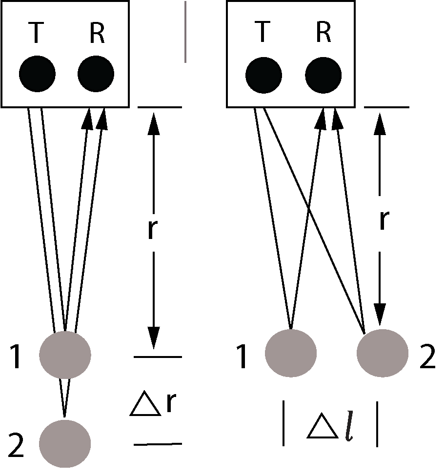
To calculate Δr and ΔƖ, the so-called vertical and lateral resolution, respectively, we need to consider the wavelength of the GPR signal, λc , which is:
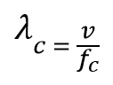
where, v is the velocity of the GPR wave in the medium and fc is the center frequency of the GPR system used.
For the GPR receiver to see two distinct objects, the second reflection must be separated enough in time from the first reflection so that the GPR receiver will see two distinct returns. For space considerations, we have skipped the derivations and are just presenting the resulting equations as follows:
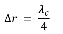
Vertical resolution is calculated by:
Horizontal resolution is calculated by:
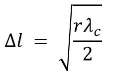
The resulting Δr and Δl values are the minimum required separation for the objects to be resolved as distinct. Notice that the vertical resolution is only dependent on the wavelength, but the horizontal (lateral) resolution is dependent on the wavelength and the depth of the targets. Essentially, the deeper you go, the worse your horizontal resolution is.
A table of horizontal and vertical resolutions for some GPR antenna center frequencies are calculated as shown below:
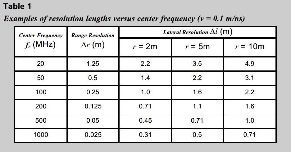
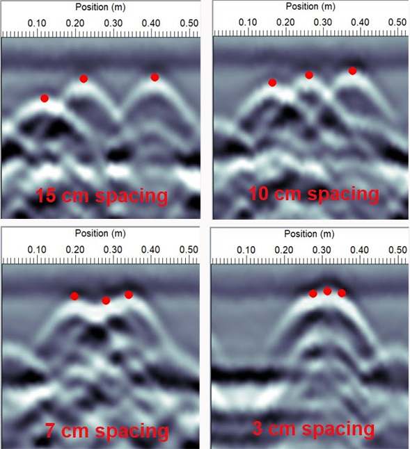
For example, we can use the lateral resolution equation to calculate the minimum horizontal separation necessary to resolve rebar when surveying with a 1000 MHz center frequency GPR system. Assuming a GPR wave velocity of 0.1 m/ns, Δl works out to 0.07m. Figure 2 shows 1000 MHz data over rebar with variable spacing. In this figure, the rebar spaced at 15 and 10 cm are clearly resolvable, the rebar with a 7 cm spacing is just resolvable (as the lateral resolution equation predicts), and the rebar with a 3 cm spacing cannot be resolved as separate objects.
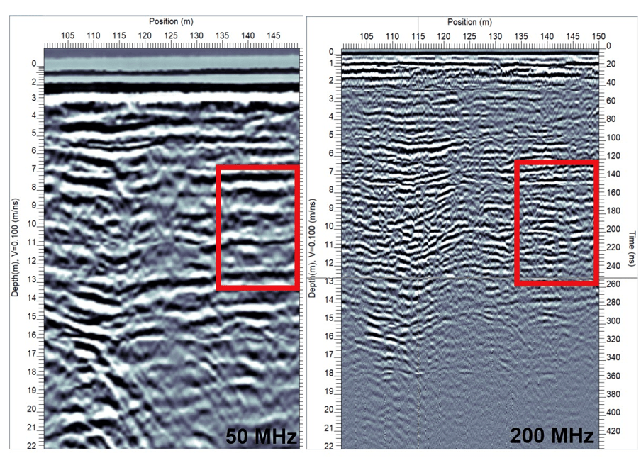
We can also use the range resolution equation to calculate the thinnest layer that can be resolved for a particular GPR antenna frequency. Figure 3 shows GPR cross sections collected at the same site with two different antennas. The higher frequency 200 MHz antenna is resolving more boundaries and thinner layers better than the lower frequency 50 MHz antenna.
A common application that requires a high resolution to measure thin layers is measuring layer thicknesses of concrete or asphalt. In the case of asphalt, layers are typically only a few centimeters thick, so high center frequency GPR systems are required to see reflections from the top and bottom of the layer to measure its thickness.
Another related application is the ability to see the bottom of a non-metallic pipe. If the reflections from the top and bottom are separated by enough time, you might see the bottom of the pipe as a distinct reflection, allowing you to estimate pipe diameter (only if you know the pipe contents). Measuring pipe diameter was covered in the January 2020 newsletter.
Keep in mind that these calculated values are theoretical. The reality is that there are other factors involved, such as background noise and clutter in the data which can make it a little harder to discern closely spaced hyperbolas or layer boundary reflections. So, use these equations to get an approximation of what to expect out in the field.
It is critical to select the proper system center frequency for your application to provide the best data. It is equally important to understand the limitations of resolution if you are looking for closely spaced targets.


