


hen interpreting GPR data where understanding geologic structure is the goal, quantifying the slope (normally referred to as ‘dip’) of interfaces is often desired. Raw GPR cross-sections are not ‘true’ representations of subsurface geometry; simplistic dip estimates will yield erroneous values for dips if the GPR wave behaviour is not considered in the calculation. The following is a very high-level summary based on simplified assumptions; this topic can get much more complex.
GPR data are normally displayed in cross-section images with a horizontal position axis and a vertical time axis (Figure 1). Time (t) is often converted to Depth (z) by knowing the wave velocity (v) in the equation:
z = vt2
where, t is the two-way travel time of the GPR wave in the subsurface.
A raw GPR cross-section display is a quick and convenient way to estimate target depths but should not be construed as a ‘true’ picture of the subsurface.
The normal expression for a dip or slope calculation is the change in depth, Δz, versus horizontal distance, Δx, along the profile, and expressed as:
θ = tan-1 ( ΔzΔx )
The slope is most often expressed as a dip angle, θ , which is the angle the interface meets the ground surface (Figure 2a). If the depths on a GPR cross-section and this expression are used to calculate the slope angle, the value will be incorrect. The reason is that the depths shown on the simple GPR cross-section are not the same as the signal ray paths in the subsurface.
These basic concepts are outlined below in Figure 2.

Figure 2a illustrates the GPR signal ray paths. The GPR transmitter and receiver are often assumed to be coincident, which is a very good approximation for most reflection surveys. The GPR signals travel in straight paths to the interface and reflect back to the GPR system. Two ray paths are shown for a GPR at positions A and B on the surface; the GPR signals reflect from the sloping interface at points A’ and B’. The lengths of the ray paths A-A’ and B-B’ are L1 and L2.
The standard GPR cross-section displays the reflected signal directly below the GPR position on the surface (Figure 2b). In fact, the signals travel a slanted or
non-vertical path to the target reflection point on the sloping surface. In a GPR cross-section, the response for path A-A’ appears at time 2L1/v and for B-B’ at time 2L1/v, where v is the GPR signal velocity in the prospected medium.

The dotted black line in Figure 2c shows the imaged reflection horizon. With the use of a simple time-to- depth conversion, Figure 2c does not change the GPR image geometry.
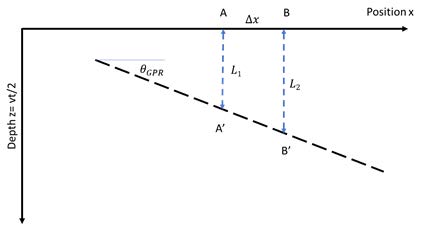
In a GPR cross-section, the sloping interface has the dip (slope), θGPR, which is related to the true interface dip, θ, as follows
tanθGPR = Slope = ΔzΔx = (L2 – L1)Δx = sinθ
The true dip can be easily computed as:
θ = sin-1 (tan θ GPR)
θ = sin-1 ( ΔzΔx )
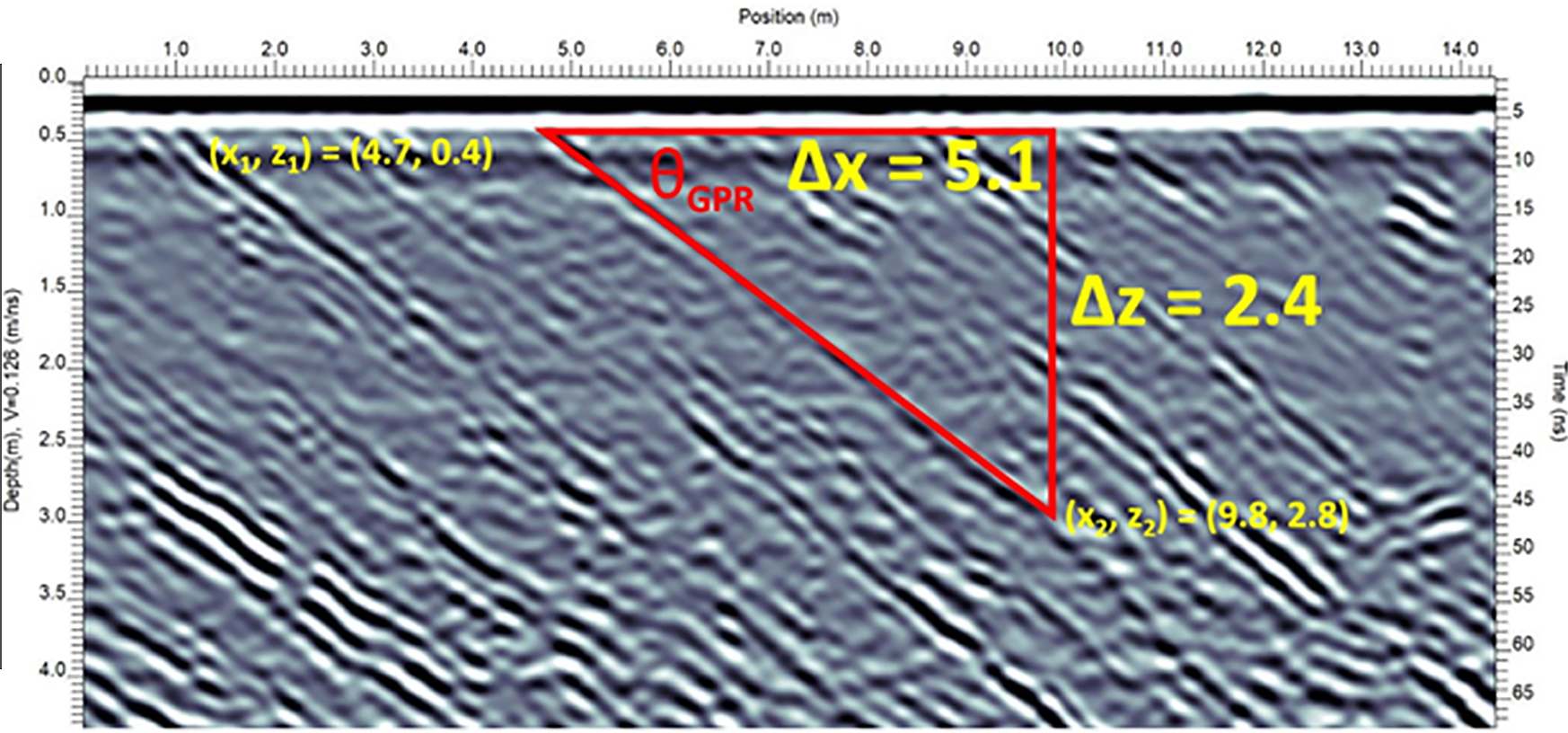
For example, using the GPR data in Figure 1:
θ = 28 degrees
Two important things to note are:
- In a simple cross-section, GPR dip, θGPR , will always be smaller than the true dip.
- The GPR image dip can only range between θ and ±45 degrees, whereas the real slope can range between θ and ±90 degrees.
Alternatively, advanced users could apply migration processing to convert the GPR section back into a true geometry cross- section. As migration moves observed ‘responses’ back to their ‘true’ location, measuring dip on a migrated section should give the correct dip. Hence migration is another way to address the true dip estimate.
This discussion is a very simple view of these concepts. In reality, the world is three dimensional and there’s no certainty that the GPR cross section is aligned with the steepest slope (this would be revealed by a GPR cross-section collected perpendicular to the strike of the structure). If a full assessment of geometry is required, it will be essential to acquire GPR data in two orthogonal directions. This ensures that the orientation of strike can be ascertained and brought into the analysis. Those details are beyond the scope of this article.
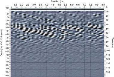
Sand dune data in Figures 1 and 3 courtesy of Todd Thompson, Indiana Geological Survey.


